Galaxy Ellipticity Distributions

This example demonstrate how to sample ellipticity distributions in SkyPy.

3D Ellipticity Distribution

In Ryden 2004 1, the ellipticity is sampled by randomly projecting a 3D ellipsoid with principal axes \(A > B > C\).

The distribution of the axis ratio \(\gamma = C/A\) is a truncated normal with mean \(\mu_\gamma\) and standard deviation \(\sigma_\gamma\).

The distribution of \(\epsilon = \log(1 - B/A)\) is truncated normal with mean \(\mu\) and standard deviation \(\sigma\).

The func:skypy.galaxies.morphology.ryden04_ellipticity() model samples projected 2D axis ratios. Specifically, it samples the axis ratios of the 3D ellipsoid according to the description above [1] and then randomly projects them using skypy.utils.random.triaxial_axis_ratio().

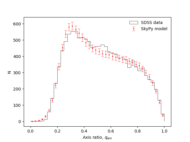
Validation plot with SDSS Data

Here we validate our function by comparing our SkyPy simulated galaxy ellipticities against observational data from SDSS DR1 in Figure 1 [1]. You can download the data file SDSS_ellipticity, stored as a 2D array: \(e_1\), \(e_2\).

import numpy as np

# Load SDSS data from Fig. 1 in Ryden 2004
data = np.load('SDSS_ellipticity.npz')
e1, e2 = data['sdss']['e1'], data['sdss']['e2']

Ngal = len(e1)
e = np.hypot(e1, e2)
q_amSDSS = np.sqrt((1 - e)/(1 + e))

In this example, we generate 100 galaxy ellipticity samples using the SkyPy function skypy.galaxies.morphology.ryden04_ellipticity() and the best fit parameters given in Ryden 2004 [1]: \(\mu_\gamma =0.222\), \(\sigma_\gamma=0.057\), \(\mu =-1.85\) and \(\sigma=0.89\).

from skypy.galaxies.morphology import ryden04_ellipticity

# Best fit parameters from Fig. 1 in Ryden 2004
mu_gamma, sigma_gamma, mu, sigma = 0.222, 0.057, -1.85, 0.89

# Binning scheme of Fig. 1
bins = np.linspace(0, 1, 41)
mid = 0.5 * (bins[:-1] + bins[1:])

# Mean and variance of sampling
mean = np.zeros(len(bins)-1)
var = np.zeros(len(bins)-1)

# Create 100 SkyPy realisations
for i in range(100):
    # sample ellipticity
    e = ryden04_ellipticity(mu_gamma, sigma_gamma, mu, sigma, size=Ngal)
    # recover axis ratio from ellipticity
    q = (1 - e)/(1 + e)
    # bin
    n, _ = np.histogram(q, bins=bins)

    # update mean and variance
    x = n - mean
    mean += x/(i+1)
    y = n - mean
    var += x*y

# finalise variance and standard deviation
var = var/i
std = np.sqrt(var)

We now plot the distribution of axis ratio \(𝑞_{am}\) using adaptive moments in the i band, for exponential galaxies in the SDSS DR1 (solid line). The data points with error bars represent the SkyPy simulation:

import matplotlib.pyplot as plt

plt.hist(q_amSDSS, range=[0, 1], bins=40, histtype='step',
         ec='k', lw=0.5, label='SDSS data')
plt.errorbar(mid, mean, yerr=std, fmt='.r', ms=4, capsize=3,
             lw=0.5, mew=0.5, label='SkyPy model')

plt.xlabel(r'Axis ratio, $q_{am}$')
plt.ylabel(r'N')
plt.legend(frameon=False)
plt.show()

References

1

Ryden, Barbara S., 2004, The Astrophysical Journal, Volume 601, Issue 1, pp. 214-220